Posted: December 4th, 2014 | Author: Gina Collecchia | Comments Off on Numbers and Notes is once more available in print
Help support me and my work on future editions of Numbers and Notes by buying a paperback copy for $16.99 $9.99 + S&H or PDF for just $1. Click here or on the button below to go to my Paypal store for the book, hosted on my personal website.
And stay tuned for Kindle and other eBook versions of the second edition of Numbers and Notes, coming February 2015!
Please email support@ginacollecchia.com should any complications arise. Happy DSP’ing!

Posted: July 16th, 2012 | Author: Gina Collecchia | Comments Off on Review featured in Keyboard Magazine!
Numbers and Notes was reviewed in the July issue of Keyboard Magazine by Stephen Fortner, Executive Editor. Check it out! 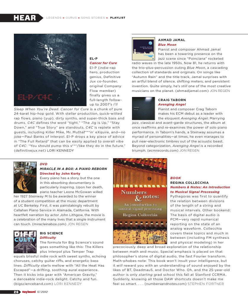
Posted: April 15th, 2012 | Author: Gina Collecchia | Comments Off on Code examples from Numbers and Notes
As promised! Download here.
Whatis: MATLAB and C examples from Appendix B of Numbers and notes. The program reads in WAVE format files so that they may be properly decoded for further analysis—the RIFF header information is read in, tossed, and the binary is converted to decimal floats. Then, computes an FFT and spits out a CSV file ready to be opened in Excel. Instructions for how to run these files is given in the book!
As for the MATLAB code, I’ve included the spectrogram maker and a simple FFT script. Remember to add this folder’s directory to your MATLAB path by going to File->Set Path…!
Happy hacking!
Posted: March 30th, 2012 | Author: Gina Collecchia | Comments Off on Stop the presses! Numbers and Notes is OUT!
Actually, on second thought, keep the presses going…
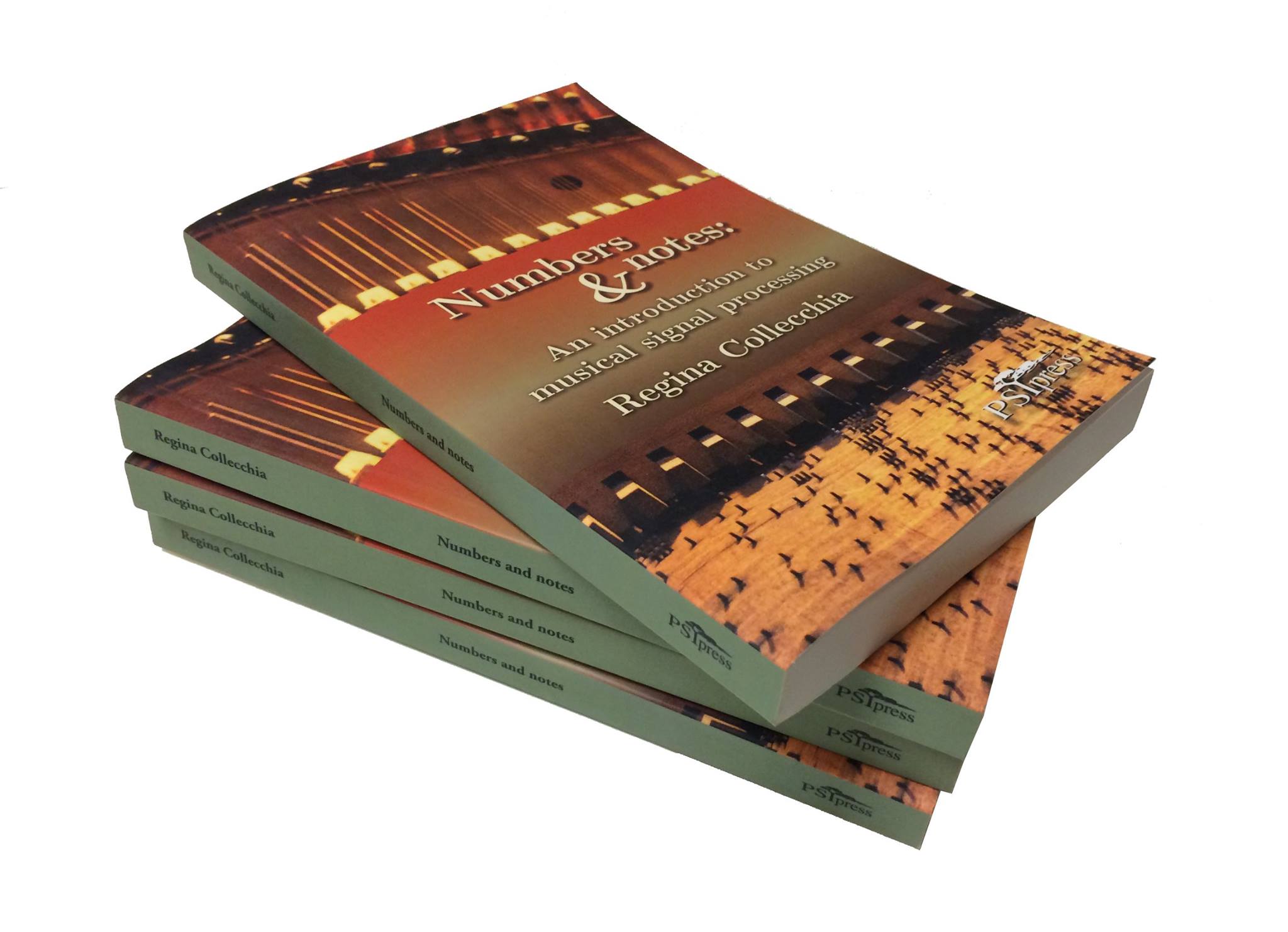
As of Monday, March 26, 2012, Numbers and notes: An introduction to musical signal processing is available on paperback, for $16.99 from Perfectly Scientific Press out of Portland, OR. I’m really happy with the way they look (and feel; the cover is made out of some weird, rubbery, smooth material).
Why should you read my book? The reasons are endless, of course! First and foremost, if you want to understand the discrete and fast Fourier transform for any application (but especially for audio purposes), this is a colloquial yet thorough introduction and clarification of the algorithm. Also included are several coding examples in C, MATLAB, and Mathematica. But in general, if you are embarking upon journeys in music information retrieval, musical instrument design, or sound recording conventions, Numbers and notes will clarify all of the underlying mathematics beneath these principles.
Numbers and notes starts from the beginning with the physics of waves and an overview of trigonometry and calculus. No more cross-referencing! Then, we move on to the digital age and uncover sampling and compression techniques. Finally, we reveal the discrete Fourier transform and its celebrated child, the fast Fourier transform, with audio applications in mind. Also addressed are the procedures for analyzing analog circuits, computing transfer functions, and designing analog and digital filters.
Numbers and notes is available in both paperback and PDF (iPad-compatible) formats. Get your copy from the Perfectly Scientific Press store.
Peek at the front and back covers (forgive that typo in the About the Author—out of my hands, out of my hands) below!


Posted: February 4th, 2012 | Author: Gina Collecchia | Comments Off on Gibbs phenomenon
is boring, so this is going to be short. Basically, Gibbs phenomenon was discovered by a guy with the last name “Gibbs” when he saw that the Fourier series of nondifferentiable waves is least-good where the waves are not differentiable. Yeah…okay. So, when a wave has sharp edges/corners like a square wave or the absolute value function, the Fourier series representation will be infinite and have these little tail thingies sticking out at these corners and edges. Honestly, it’s not that surprising.

These thingies are called “Gibbs horns” or “Gibbs’ horns” or if the writer just hates checking Wikipedia, “Gibb’s horns,” and the points at which they exist are usually called “jump discontinuities,” i.e., sharp edge corner things.
Posted: October 14th, 2011 | Author: Gina Collecchia | Comments Off on A (super short) introduction to acoustic physical modeling
What does it take to understand the acoustics of a physical space, like a room or a musical instrument? You don’t have to be a musician to desire—or even require—good sound. The acoustics of an amphitheater or simple rectangular room dictate the the signal-to-noise ratios of sonic signals like speech and music. When sound reflects off of the walls, ceiling, floor, and other objects in a room, it loses energy (volume) each time it does so. In highly reverberant rooms such as churches (the Hagia Sophia in Turkey has something like a 10-second reverberation time!), the reflections are numerous because they don’t lose as much energy with each bounce, so signals originating from the space will retain less information because previous signals are still bouncing around. So, the greater the reverberation, the less signal and greater noise.
But, not all signals are equal. Acoustic spaces (and musical instruments) are ideally designed to give preferences to a certain frequency range, which for speech is about 1000-5000 Hz. We can test these “frequency preferences” by measuring how the room behaves to specific frequencies. This measurement is called a frequency response. One way to do this is by playing a sine sweep—a sine wave starting from 0 Hz and constantly increasing (linearly or logarithmically) until ending at 25000 Hz (or whatever desired range)—and recording it in the room. This method requires no transformation to a frequency domain because time and frequency are tied! The recorded amplitude is the amplitude response of the room. From this, it should be clear that a room and a musical instrument alike are both types of filters.
However, speakers have frequency responses, too, so unless that response is known (and even if it is), the sine sweep can pose problems and return inaccuracies. Fortunately, there is another, more clever way to do this: by an impulse function, such as one of those mentioned in the post below. Refresher: an impulse function \delta(t-a) is defined as zero everywhere that t does not equal a (t is time, a is some instant of time), and non-zero where t=a (infinity in the continuous case and 1 in the discrete case). An impulse function is not differentiable, but it is integrable (in the continuous case), and its integral is equal to 1.
Now, what does an impulse sound like? This two-fold jump in amplitude from 0 to maximum value to 0 again is colloquially called a tone burst: it’s like dropping the needle on a record player, or sampling audio at non-zero endpoints and causing a speaker to emit a ‘click’—the sound of it trying to move infinitely fast (because velocity is the derivative of position! So it all comes down to differentiability!) from one position to another. This is also known as clipping, an undesirable effect in virtually every aspect of life save hygiene (okay, there may exist others). What does clipping have to do with the frequency responses of acoustic spaces? Well, what is the frequency response of an impulse?
This is quickly calculated by taking the Fourier transform of \delta(t-a), which is equal to exp(-ia\omega), where \omega is frequency. When a=0, which is the case for a single impulse, and since time is relative (don’t sue; yeah I’ve seen the article about the neutrinos), it’s okay to call a=0 in most situations. Thus, F{\delta(t-0)}=exp(-i0\omega)=1 for all \omega. This is called a flat (frequency) response, the desired response for speakers, and when we apply it to a room and record the results, the Fourier transform of the results shows the frequency response of the room!
The sound of an impulse is that of white noise, which has equal energy spread to all frequencies, much like white light contains the entire visible spectrum. The Fourier transform of \delta(t-a) is exp(-ia\omega) because of the Shifting theorem, which states that F{x(t-a)}=F{x(t)}*exp(-ia\omega). Finally, the Fourier transform of a finite-time-domain signal is infinite, and the Fourier transform of an infinite-time-domain signal is finite. This is a result of Gibb’s Phenomenon, the subject of my next post!
Happy DSP’ing!
Posted: August 25th, 2011 | Author: Gina Collecchia | Comments Off on Kronecker vs. Dirac delta functions
Delta functions are used to sample time-domain signals in signal processing, but their type is often unstated or incorrectly specified. A Dirac delta function is a continuous function d(t-a) whose integral is exactly equal to 1 and is only nonzero at t=a. Hence, it is infinitesimal in width (its width approaches 0) and infinitely tall (its amplitude approaches infinity). The Dirac delta is applied to analog, continuous signals to return a continuous scaled impulse function at a specified instant of time (indicated by the domain of the Dirac delta). This is done by taking the integral over all values of the signal x(t) times the Dirac delta centered at a, d(t-a). The resulting function is a continuous function equal to x(a)*d(t-a).
The Kronecker delta function is similarly infinitesimally thin, but its amplitude is equal to 1, not its area. The function d[t-a] is equal to 1 when t=a and 0 otherwise, i.e., when t!=a. The Kronecker delta is a discrete function. It applies a discrete impulse to a continuous signal, and returns the original amplitude of the signal. Therefore, the resulting function is discrete, and equal to x[a]*d[t-a].
Since they can be written the same way (the square brackets to indicate that a function is discrete are not required), most texts will just call the delta function the Dirac type, if any. But if this were so, a discrete signal would have all infinite (positively and negatively) amplitudes! So, the difference is significant.
Wish I could have TeX’ed that but hopefully you found this helpful. The concept of a sampled function is really what is important here, and it represents the amplitude of a continuous signal at specific points of time. But a Dirac returns a continuous sampled function, and a Kronecker returns a discrete one.
Posted: November 16th, 2010 | Author: Gina Collecchia | Comments Off on Reed my thesis!
A great read. Be nice.
Posted: August 26th, 2010 | Author: Gina Collecchia | Comments Off on The “Greek” modes
You may have overheard some of your more bookish friends attempting to one-up your certainly basic understanding of music theory by referring to the Greek modes. But here’s an interesting fact: the Ionian, Dorian, Phrygian, etc. modes are not actually the modes originally used by the Greeks.
The history of how exactly they have developed into variations of our familiar Western 12-tone scale is muddied by many writings from Europe between the 6th and 9th century. Furthermore, half of the modes might have been plagal, meaning they were completed by the addition of lower notes instead of higher ones (in which case the mode is called authentic), like the Gregorian modes. Either way, the modes would better be called “medieval” or “church” modes, as they were predominantly used in the time of Pope Gregory I, in the Roman Catholic church during the 10th-13th centuries.
So, the next time some hipster asks you what Greek mode the new Iron and Wine single is in, first answer Ionian or Aeolian, and then sock it to them.
Posted: June 10th, 2010 | Author: Gina Collecchia | Comments Off on Call for synesthetes
(1) “…Synesthetes will reveal a systematic relationship between color brightness or lightness and auditory pitch: The higher the pitch of the sound, the lighter or brighter the color of the image.”
(2) “The higher the pitch of the sound, the sharper, more angular, and smaller the visual image.”
(3) “Synesthetic images are typically simple (e.g., color or shape), but dynamic (e.g., as the sound waxes and wanes, so does the image). In some cases, the induced image is so vivid as to be distracting.”
All of these quotes come from the fascinating article “Synesthesia: Strong and Weak” by Martino & Marks (view the JSTOR article, available through your public library account).
I am in need of candidates who possess any kind of synesthetic gift, realized or unrealized, weak or strong, preferably with respect to pitch detection. A friend of mine in high school would see specific colors for specific pitches. That is not to say that perfect (absolute) pitch requires synesthetic qualities, but I would like to know if those with strong or weak synesthesia have a proclivity for identifying pitches in isolation.
I am also very interested in talking with people who have absolute pitch without synesthesia, and those who have amusia or are tone deaf.
Contact me at info[at]numbersandnotes[dot]com. You will be contacted with a questionnaire or a phone interview, and you may even be compensated for your time.


